TL;DR

You’ll discover how to apply IFRS 13 valuation techniques with clarity and confidence. This guide walks you through the market approach, income approach, and cost approach in practical terms. You’ll master fair value measurement challenges, understand valuation adjustments, and learn the fair value hierarchy levels. You’ll also calibrate models, combine techniques effectively, and understand disclosure requirements that matter to auditors. Whether you’re managing asset valuations locally or internationally, this article gives you compliant, practical steps to strengthen your reporting. Ready to apply IFRS 13 today?

Why IFRS 13 Valuation Techniques Matter for Your Financial Reporting

You’re staring at your balance sheet, wondering if your asset valuations meet IFRS 13 requirements. You’re not alone. As of 2024, the IFRS Foundation has complete jurisdiction profiles for 169 jurisdictions worldwide, and businesses across these regions face the same challenge.

Fair value measurement isn’t just a compliance checkbox. It’s the foundation of transparent financial reporting that investors, regulators, and stakeholders rely on. IFRS 13 was issued in May 2011 and includes all amendments issued through December 31, 2024, setting the global standard for how you value assets and liabilities.

This guide breaks down IFRS 13 valuation techniques into actionable steps you can implement right away. You’ll learn when to use each approach, how to calibrate your techniques, and what pitfalls to avoid. Whether you’re operating locally or across multiple regions, these principles will help you strengthen your financial reporting and pass auditor scrutiny.

Understanding IFRS 13 Valuation Techniques and Input Levels

IFRS 13 defines fair value as an exit price. That’s the price you’d receive to sell an asset or pay to transfer a liability in an orderly transaction between market participants at the measurement date.

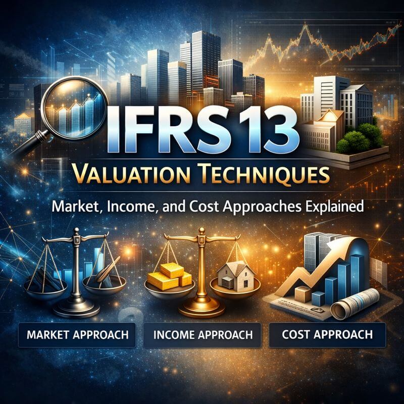
Three families of IFRS 13 valuation techniques form the core of this standard.

The market approach uses prices and data from actual market transactions involving similar assets or liabilities. You’ll see this with business multiples and matrix pricing for bonds.

The income approach converts future amounts into a single discounted present value. Think discounted cash flows, option pricing models, and multi-period excess earnings methods.

The cost approach represents the amount needed to replace an asset’s service capacity. It’s often called current replacement cost, adjusted for obsolescence.

Your goal is straightforward: maximize observable inputs and minimize unobservable ones. This principle runs through every valuation decision you make.

Input reliability matters significantly. A 2020 study examining 277 auditors across post-IFRS 13 implementation identified the most critical challenge: insufficient data for valuing items. This shortage of reliable data affects organizations across all regions.

When you select a valuation technique, you must ensure adequate data supports your choice. The standard doesn’t mandate one technique over another. You can use multiple approaches when appropriate. What matters is consistency and appropriateness for your specific circumstances.

Fair Value Hierarchy Levels: Why Each Level Matters

The fair value hierarchy ranks inputs into three levels based on observability and reliability.

Level 1 inputs are quoted prices in active markets for identical assets or liabilities. These are unadjusted prices you can access at the measurement date. They’re the gold standard because they provide the most reliable fair value evidence. You must use Level 1 inputs whenever available, with very limited exceptions.

Level 2 inputs are observable but not quoted prices. They include quoted prices for similar assets in active markets, quoted prices for identical or similar assets in inactive markets, and inputs corroborated by market data. Interest rate curves, credit spreads, and foreign exchange rates typically fall here.

Level 3 inputs are unobservable. You develop these based on the best information available, reflecting assumptions market participants would use. Management forecasts, internal pricing models, and proprietary data often create Level 3 inputs.

The level you assign isn’t about the valuation technique itself. It’s about the inputs you use. A discounted cash flow model using observable discount rates might be Level 2, while the same model with unobservable inputs becomes Level 3.

Here’s what matters: your fair value measurement gets classified based on the lowest level input that’s significant to the entire measurement. One significant unobservable input can push your entire valuation into Level 3.

Measurement Inputs: Observable vs. Unobservable

Observable inputs come from market data independent of your reporting entity. They reflect assumptions market participants would use and are generally more reliable than unobservable inputs.

Unobservable inputs reflect your own assumptions about what market participants would consider. You develop these when observable inputs aren’t available. Think internal forecasts, adjusted industry benchmarks, or proprietary models.

The standard requires you to take into account all information about market participant assumptions that’s reasonably available. You don’t need exhaustive efforts, but you can’t ignore readily available data either.

The At-Arms-Length Principle in Fair Value Measurement

Fair value assumes an orderly transaction between market participants. That means willing buyers and sellers who are independent, knowledgeable, and able to transact.

You’re not measuring forced liquidation values or distressed sale prices. The transaction should reflect normal market conditions and motivations. Market participants act in their economic best interest.

This principle affects how you adjust for premiums and discounts. A control premium might apply if market participants would pay extra for control. A blockage discount generally doesn’t apply because you measure fair value for the unit of account, not a larger block.

Market Approach: How to Apply Observable Market Data in IFRS 13 Valuations

The market approach uses prices from comparable transactions. You’re looking at what similar assets or liabilities actually trade for in the market.

Start by identifying comparable transactions. Look for similar assets in terms of characteristics, risks, and cash flow patterns. Industry, size, growth prospects, and market conditions should align.

Business valuation multiples are common market approach applications. You might use revenue multiples, EBITDA multiples, or price-to-earnings ratios from comparable public companies or transactions. The key is adjusting these multiples for differences between your subject and the comparables.

Matrix pricing works well for fixed income securities. You create a matrix of similar securities arranged by key features like credit rating, maturity, and industry. Then you interpolate to estimate your security’s fair value.

Recent transaction prices for the same or similar items provide strong evidence. But you need to consider whether those transactions were orderly and whether circumstances have changed.

Adjustments are usually necessary. No two assets are identical. You’ll adjust for differences in condition, location, marketability, and other relevant factors. Each adjustment should reflect what market participants would consider.

When applying the market approach to IFRS 13 asset valuation, you must document your comparability analysis and adjustment rationale. Transparency matters for both internal decision-making and external audit.

Income Approach: Converting Future Cash Flows into Present Value

The income approach focuses on future economic benefits. You’re converting expected future amounts into a single present value.

Discounted cash flow (DCF) analysis is the most common income approach technique. You project future cash flows and discount them back to present value using an appropriate discount rate.

Start with cash flow projections. These should reflect market participant expectations, not just your internal plans. Consider multiple scenarios when relevant. Expected cash flows represent probability-weighted averages of possible outcomes.

Your discount rate must match the risk inherent in the cash flows. If you use expected (probability-weighted) cash flows, your discount rate should reflect only systematic risk. If you use management’s best estimate (a single scenario), you might need to add a company-specific risk premium.

Two main present value techniques exist under IFRS 13. The discount rate adjustment technique uses a single set of cash flows (often contractual or most likely) with a risk-adjusted discount rate. The expected cash flow technique uses probability-weighted cash flows with a risk-free or risk-adjusted rate.

Option pricing models apply when assets or liabilities have option-like features. Black-Scholes, binomial models, and Monte Carlo simulations can value these features. You’ll use these for convertible securities, contingent consideration, or complex derivatives.

The multi-period excess earnings method values intangible assets. It isolates cash flows attributable to the specific intangible, charging for contributory assets used alongside it. This technique is common in business combination accounting.

Calibration: Connecting Your Valuation to Market Reality

Calibration is critical. At initial recognition, if your income approach doesn’t equal the transaction price, you need to calibrate your unobservable inputs. Calculate the implied internal rate of return or adjust your growth assumptions to match.

This step bridges the gap between your model and what the market actually paid. It’s not about changing your methodology—it’s about refining your assumptions to reflect market reality.

Impact of Valuation Choices on Financial Reporting and Key Ratios

Your valuation technique choices affect reported earnings, equity, and key financial ratios. Level 3 measurements, which rely heavily on the income approach, introduce more volatility and subjectivity.

Fair value changes flow through profit or loss or other comprehensive income, depending on the accounting standard governing the item. This creates earnings volatility, especially for financial instruments at fair value through profit or loss.

Debt-to-equity ratios, return on assets, and earnings per share all shift with fair value adjustments. Stakeholders watch these metrics closely. Your valuation methodology directly impacts their assessment of your financial health.

Conservative income approach assumptions might understate asset values, improving future performance when those assets perform better than expected. Aggressive assumptions create the opposite effect.

Cost Approach: Understanding Replacement and Reproduction Cost Methods

The cost approach asks: what would it cost to replace this asset’s service capacity?

You’re measuring current replacement cost, adjusted for obsolescence. This technique assumes a rational market participant wouldn’t pay more for an asset than the cost to acquire or construct a substitute with comparable utility.

Replacement cost differs from reproduction cost. Replacement cost is the cost to acquire a substitute asset of comparable utility using modern materials and technology. Reproduction cost is the cost to replicate the exact asset.

Replacement cost is usually more relevant because market participants would use current technology and materials. Reproduction makes sense only when the specific characteristics matter and substitutes don’t exist.

Physical deterioration reduces value below replacement cost. Age, wear, and maintenance history all matter. You’ll typically see this in property, plant, and equipment valuations.

Functional obsolescence occurs when design features make the asset less useful than modern alternatives. Excess operating costs, inadequate capacity, or outdated technology create functional obsolescence.

Economic obsolescence comes from external factors. Changes in demand, regulation, or competitive landscape can reduce an asset’s value even if it’s physically sound and functionally adequate.

The cost approach sees less frequent use than market and income approaches. But it’s valuable for specialized assets with limited market data, assets under construction, and certain intangible assets like internally developed software.

When you apply the cost approach, document your obsolescence adjustments carefully. These require significant judgment and market participants might view them differently.

Calibrating IFRS 13 Valuation Techniques to Transaction Prices

Calibration ensures your valuation technique reflects transaction prices at initial recognition. This step is mandatory when you’ll fair value the item going forward and your technique uses unobservable inputs.

Here’s why calibration matters: your unobservable inputs might not reflect market participant assumptions. The transaction price provides evidence of what market participants actually paid.

For example, you acquire an unquoted equity interest for $10 million. Your DCF model using your internal assumptions values it at $8 million. You need to calibrate. Either your cash flow projections are too conservative, your discount rate is too high, or your growth assumptions are too low.

Calculate the implied internal rate of return that makes your DCF equal the transaction price. Use that IRR as your discount rate going forward, assuming market conditions haven’t changed.

For market approach calibrations, you might adjust premiums or discounts applied to comparable company multiples. If comparable companies trade at 8x EBITDA but your transaction occurred at 10x, you need to understand and document that premium.

Calibration isn’t one-time. You recalibrate when you change valuation techniques or when market conditions change significantly. Document your calibration process and maintain it consistently.

The standard gives specific guidance for calibrating premiums and discounts, particularly relevant for unquoted equity interests. You isolate the factors that explain the difference between the transaction price and your initial model output.

Using Multiple IFRS 13 Valuation Techniques: Best Practices and Weighting

Sometimes one technique isn’t enough. Multiple approaches provide better evidence of fair value, especially for complex items or when markets are inactive.

When should you use multiple techniques? Consider it when no single approach clearly dominates, when different techniques provide conflicting results you need to reconcile, or when market conditions create uncertainty.

Weight your techniques based on their reliability and relevance. If you have recent comparable transactions, weight the market approach heavily. If markets are inactive but you have solid cash flow projections, emphasize the income approach.

Reconcile differences between techniques. If your DCF gives you $15 million but comparable multiples suggest $12 million, investigate why. Market conditions, company-specific factors, or input errors could explain the gap.

Document your weighting rationale. Auditors and stakeholders will ask why you chose one result over another. Clear documentation of your thought process demonstrates proper application of IFRS 13 valuation techniques.

Multiple techniques don’t mean averaging results mechanically. You’re not calculating arithmetic means. You’re using professional judgment to determine which technique or combination best reflects fair value in your circumstances.

Consistency matters. If you use multiple techniques for an asset class, apply that approach consistently unless circumstances change. IFRS 13 paragraph 65 allows changes when they result in equally or more representative fair value measurements.

Common Challenges and Pitfalls in IFRS 13 Fair Value Measurements

The 2020 audit study identified several post-implementation challenges: manipulation of asset and liability values with no market price during estimation, managers using non-availability of market information to manipulate financial statements, and inappropriateness or non-compliance of valuation methods with IFRS 13.

Inactive markets create significant challenges. When transaction volume drops, quoted prices might not reflect orderly transactions. You’ll need to adjust or supplement quoted prices with other valuation techniques.

Unit of account issues confuse many practitioners. Are you valuing an individual instrument or a portfolio? The answer affects which practical expedients you can use and how you apply valuation techniques.

Non-performance risk, including credit risk, must be considered for liabilities. Many practitioners overlook this requirement. Your own credit risk affects the fair value of your liabilities.

Day one gains or losses require careful consideration. When transaction price differs from fair value at initial recognition, you might recognize an immediate gain or loss. But IFRS 13 creates a rebuttable presumption that transaction price equals fair value.

Overlooking market participant assumptions is another common error. Your internal assumptions don’t matter unless market participants would share them. Always ask: what would a typical market participant assume?

Changes in valuation techniques need proper justification. You can’t switch techniques just because you prefer the result. The change must produce equally or more representative fair value measurements.

For IFRS 13 fair value measurement challenges, understanding comparative valuation techniques and when to apply each one is critical to compliance and accuracy.

IFRS 13 Disclosure Requirements for Fair Value Measurements

Disclosure requirements vary based on the fair value hierarchy level and whether measurements are recurring or non-recurring.

Recurring measurements occur at each reporting date. Financial instruments at fair value and investment property under the fair value model are typical examples.

Non-recurring measurements happen in specific circumstances. Assets classified as held for sale, impairment testing, and contingent consideration are common triggers.

For all fair value measurements, you must disclose the fair value measurement at the end of the reporting period and the level within the fair value hierarchy. You’ll also disclose the reasons for any transfers between hierarchy levels.

Transparency and Disclosure: What Auditors and Regulators Expect

Level 1 disclosures are relatively straightforward. You confirm you used quoted prices in active markets and disclose the level in the hierarchy.

Level 2 requires more detail. Disclose the valuation techniques and inputs used. Describe how you determined fair value. If you changed techniques, explain why.

Level 3 demands extensive disclosure. You must provide a reconciliation of opening and closing balances, showing gains and losses recognized, purchases, sales, and transfers. For recurring measurements, disclose the effect on profit or loss or other comprehensive income.

Quantitative information about significant unobservable inputs is required for Level 3. You can’t just name the inputs—you must quantify them.

Sensitivity analysis applies to recurring Level 3 financial instrument measurements. You disclose how changes in unobservable inputs would affect fair value. But this requirement has exceptions: if changing inputs wouldn’t significantly affect fair value, no disclosure is needed.

For non-financial assets measured at fair value, disclose whether you’re using the asset’s current use or highest and best use. If they differ, explain why and the financial impact.

You must describe the valuation processes used. Who performs valuations? What qualifications do they have? How often do you review and update assumptions?

Related party relationships can affect fair value. If you transacted with related parties, that context matters for understanding whether the transaction was orderly.

Practical Examples of IFRS 13 Valuation Techniques in Action

Let’s see how these techniques work in real scenarios.

Example 1: Valuing Unquoted Equity Interests Using Market Multiples

You hold a 25% interest in a private company. Comparable public companies trade at 6-8x EBITDA. Your investee’s EBITDA is $5 million. You identify three comparable public companies with an average multiple of 7x EBITDA.

Before applying the multiple, you adjust for differences. Your investee is smaller, less liquid, and you lack control. You apply a 20% discount for lack of marketability and a 15% discount for minority interest. The calculation: $5 million x 7x x 25% = $8.75 million, less 35% combined discount = $5.69 million fair value.

You calibrate this at initial acquisition. If you paid $6 million, you recalculate the implied discount at 14.3%, which becomes your ongoing discount assumption unless market conditions change.

Example 2: DCF Valuation for Investment Property

You own a commercial building generating $1 million annual net rent. Market data suggests a 7% capitalization rate for similar properties. Using the income approach: $1 million / 7% = $14.3 million fair value.

You also check recent sales of comparable properties (market approach). Similar buildings sold for $13.8-$14.5 million. This corroborates your income approach result. You determine fair value is $14.3 million based on both techniques.

Example 3: Contingent Consideration in Business Acquisition

You acquired a business and agreed to pay an additional $2 million if EBITDA exceeds $8 million within two years. You estimate a 60% probability of achieving this target.

Simple expected value: $2 million x 60% = $1.2 million. But you need to discount this to present value using a rate that reflects the risk. If the appropriate discount rate is 10%, the present value is approximately $991,000.

You’d classify this as Level 3 because the probability estimate is unobservable. You’d disclose your valuation technique, key inputs (probability and discount rate), and sensitivity to changes in those inputs.

How to Choose the Right Valuation Technique in Complex Scenarios

Selection starts with understanding your asset or liability. What’s the unit of account? What characteristics matter to market participants?

Consider data availability. The best technique theoretically means nothing if you can’t obtain reliable inputs. Level 1 inputs trump sophisticated models with Level 3 inputs.

Match the technique to the item’s characteristics. The market approach works best when comparable transactions exist. Income approaches suit assets generating cash flows. Cost approaches fit specialized assets with limited market data.

Market conditions influence your choice. Active markets support market approaches. Inactive markets might require income or cost approaches.

For complex financial instruments with embedded derivatives, you might need specialized models. Option pricing techniques, Monte Carlo simulations, or lattice models could apply.

Investment property valuation typically combines income approach (capitalization of net operating income) with market approach (comparable sales). Real estate markets often provide data for both techniques.

Intangible assets acquired in business combinations frequently use the multi-period excess earnings method (income approach). This isolates cash flows attributable to the specific intangible.

When you’re uncertain which technique is most appropriate, pilot multiple approaches. Compare results. Understand why they differ. This analysis helps you determine which technique best reflects fair value in your situation.

Document your selection process. Explain why you chose one technique over alternatives. This documentation supports audit trails and helps maintain consistency.

For organizations operating internationally, consider regional market differences. Market liquidity, available comparables, and data sources vary by jurisdiction. Your IFRS advisory services provider should understand these regional nuances.

Recent research shows that IFRS 17 insurance contracts implementation saw 46% of companies experience downside effects on shareholders’ equity due to increased insurance liabilities. Similar fair value measurement challenges apply across standards, affecting how companies approach IFRS 13 asset valuation and valuation risk management.

Looking ahead, fair value measurement continues to expand. ASU 2023-08 requires in-scope crypto assets to be measured at fair value, effective for annual and interim periods in fiscal years beginning after December 15, 2024, with early adoption permitted. This shows how fair value frameworks adapt to new asset classes.

Master IFRS 13 Valuation Techniques with Confidence and Clarity

You now have a roadmap for applying IFRS 13 valuation techniques. From understanding input hierarchies to calibrating your models, each step builds toward accurate, compliant financial reporting.

The market approach gives you real transaction evidence. The income approach captures future economic benefits. The cost approach grounds you in replacement economics. Use them individually or in combination, always maximizing observable inputs.

Fair value hierarchy levels guide your disclosure requirements. Level 3 measurements demand extensive transparency about your unobservable inputs and assumptions. Don’t underestimate the documentation burden.

Calibration connects your models to market reality. When transaction prices diverge from your initial estimates, recalibrate your inputs to reflect market participant assumptions.

Prima Consulting’s IFRS 13 valuation services bring decades of combined experience helping organizations implement IFRS 13 valuation techniques. Our team understands market conditions, regulatory requirements, and global best practices. We’ll partner with you to build robust valuation frameworks that withstand audit scrutiny and support confident decision-making.

Ready to strengthen your fair value measurement process? Contact Prima Consulting today to discuss how we can help you master IFRS 13 implementation and achieve compliance confidence.